

Reading and analyzing data with Neo#
Getting started#
Neo is a library for working with neurophysiology data in the Python programming language. One of the big advantages of Neo is that it works with many different file formats: it doesn’t matter which format your data is stored in, Neo provides a standard way to read the data, and then represents it in a standardised way, as a set of Python objects.
The first step in reading data is to import the appropriate Neo input-output (or IO) module for your data.
For this example, we’re going to work with membrane potential traces stored in a text file,
so we use the AsciiSignalIO module:
In [1]: from neo.io import AsciiSignalIO

In [2]: data = AsciiSignalIO("example_data.txt", delimiter=" ").read()
Note
For a full list of IO modules provided by Neo, see List of implemented IO modules.
In [3]: data
Out[3]:
[Block with [<neo.core.segment.Segment object at 0x787265057e90>] segments
 file_origin: 'example_data.txt'
 # segments (N=[<neo.core.segment.Segment object at 0x787265057e90>])
 0: Segment with [<AnalogSignal(array([[-58.46900177, -52.85499954, -58.79000092, -58.81499863],
       [-59.06100082, -50.51800156, -52.00299835, -57.24000168],
       [-59.00999832, -50.50999832, -51.98799896, -57.19900131],
       ...,
       [-56.53499985, -56.65299988, -56.37400055, -53.6590004 ],
       [-56.50099945, -56.61999893, -56.41999817, -53.63999939],
       [-56.4679985 , -56.58599854, -56.4640007 , -53.62099838]],
      shape=(10001, 4)) * mV, [0.0 s, 10.001 s], sampling rate: 1.0 kHz)>] analogsignals
    # analogsignals (N=[<AnalogSignal(array([[-58.46900177, -52.85499954, -58.79000092, -58.81499863],
       [-59.06100082, -50.51800156, -52.00299835, -57.24000168],
       [-59.00999832, -50.50999832, -51.98799896, -57.19900131],
       ...,
       [-56.53499985, -56.65299988, -56.37400055, -53.6590004 ],
       [-56.50099945, -56.61999893, -56.41999817, -53.63999939],
       [-56.4679985 , -56.58599854, -56.4640007 , -53.62099838]],
      shape=(10001, 4)) * mV, [0.0 s, 10.001 s], sampling rate: 1.0 kHz)>])
    0: AnalogSignal with 4 channels of length 10001; units mV; datatype float64
       name: 'multichannel'
       sampling rate: 1.0 kHz
       time: 0.0 s to 10.001 s]
Different data files can contain different amounts of data, from single traces to multiple
recording sessions. To provide consistent behaviour, for all IO modules, the read() method returns a list of data blocks.
A Block typically represents a recording session.
Each block contains a list of segments, where each Segment contains data recorded at the same time.
In this example file, we see a single type of data, the “analog signal”, which represents continuous time series
sampled at a fixed interval. The other types of data that can be contained in a Segment are discussed below
under Data types.
Note
read() reads the entire file into memory at once. If you only want to access part of the data,
you can do so using Neo’s “lazy” data loading - see the section on Performance and memory consumption below.
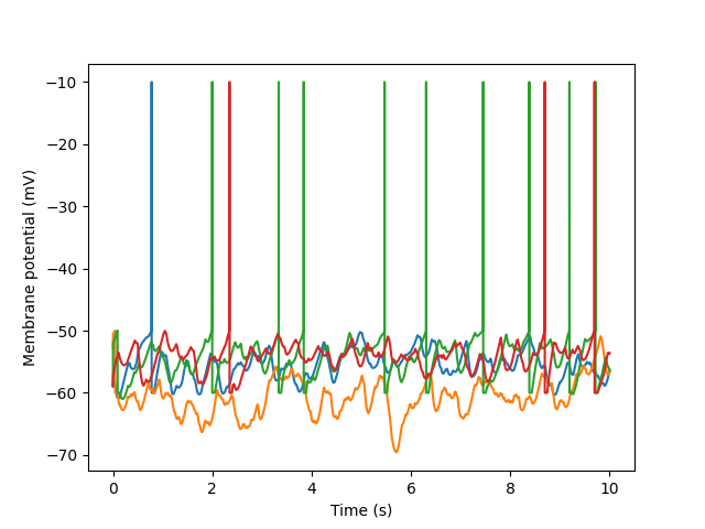
Neo data objects are based on NumPy arrays, and behave very similarly. For example, they can be plotted just like arrays:
In [4]: import matplotlib.pyplot as plt

In [5]: signal = data[0].segments[0].analogsignals[0]

In [6]: plt.plot(signal.times, signal)
Out[6]:
[<matplotlib.lines.Line2D at 0x787264955b10>,
 <matplotlib.lines.Line2D at 0x787264902990>,
 <matplotlib.lines.Line2D at 0x787264740e90>,
 <matplotlib.lines.Line2D at 0x787264903b50>]

In [7]: plt.xlabel(f"Time ({signal.times.units.dimensionality.string})")
Out[7]: Text(0.5, 0, 'Time (s)')

In [8]: plt.ylabel(f"Membrane potential ({signal.units.dimensionality.string})")
Out[8]: Text(0, 0.5, 'Membrane potential (mV)')

In [9]: plt.savefig("example_plot.png")
You now know enough to start using Neo. For more examples, see Examples. If you want to know more, read on.
NumPy#
Neo is based on NumPy. All Neo data classes behave like NumPy arrays, but have extra functionality.
The first addition is support for units.
In contrast to a plain NumPy array, an AnalogSignal knows the units of the data it contains, e.g.:
In [10]: signal.units
Out[10]: array(1.) * mV
This helps avoid errors like adding signals with different units, lets you auto-generate figure axis labels, and makes it easy to change units, like here from millivolts to volts e.g.:
In [11]: signal.magnitude[:5]
Out[11]:
array([[-58.46900177, -52.85499954, -58.79000092, -58.81499863],
       [-59.06100082, -50.51800156, -52.00299835, -57.24000168],
       [-59.00999832, -50.50999832, -51.98799896, -57.19900131],
       [-58.95999908, -50.50299835, -51.97299957, -57.15800095],
       [-58.9109993 , -50.49499893, -51.95800018, -57.11700058]])

In [12]: signal.rescale("V").magnitude[:5]
Out[12]:
array([[-0.058469, -0.052855, -0.05879 , -0.058815],
       [-0.059061, -0.050518, -0.052003, -0.05724 ],
       [-0.05901 , -0.05051 , -0.051988, -0.057199],
       [-0.05896 , -0.050503, -0.051973, -0.057158],
       [-0.058911, -0.050495, -0.051958, -0.057117]])
The second addition is support for structured metadata.
Some of these metadata are required.
For example, an AnalogSignal must always have a sampling_rate attribute,
and Neo will produce an Exception if you try to add two signals with different sampling rates:
In [13]: signal.sampling_rate
Out[13]: array(1.) * kHz
Some of these metadata are recommended but optional, like a name for each signal. Such metadata appear as attributes of the data objects:
In [14]: signal.name
Out[14]: 'multichannel'
And finally, some metadata are fully optional.
These are stored in the annotations and array_annotations attributes:
In [15]: signal.array_annotations
Out[15]: {'channel_index': array([0, 1, 2, 3])}
For more information about this, see Annotations.
Most NumPy array methods also work on Neo data objects, e.g.:
In [16]: signal.mean()
Out[16]: array(-56.33598084) * mV
Data objects can be sliced like arrays (array annotations are automatically sliced appropriately):
In [17]: signal[100:110, 1:3]
Out[17]:
AnalogSignal with 2 channels of length 10; units mV; datatype float64
name: 'multichannel'
sampling rate: 1.0 kHz
time: 0.1 s to 0.11 s

In [18]: signal[100:110, 1:3].array_annotations
Out[18]: {'channel_index': array([1, 2])}
To convert a Neo data object to a plain NumPy array, use the magnitude attribute:
In [19]: signal[100:110, 1:3].magnitude
Out[19]:
array([[-60.65399933, -60.        ],
       [-60.72399902, -60.        ],
       [-60.79199982, -60.        ],
       [-60.85900116, -60.        ],
       [-60.92399979, -60.        ],
       [-60.98899841, -60.        ],
       [-61.05199814, -60.        ],
       [-61.11399841, -60.        ],
       [-61.17499924, -60.        ],
       [-61.23400116, -60.        ]])
Data types#
The following classes directly represent data as arrays of numerical values with associated metadata (units, sampling frequency, etc.).
AnalogSignal: A regular sampling of a single- or multi-channel continuous analog signal.
IrregularlySampledSignal: A non-regular sampling of a single- or multi-channel continuous analog signal.
SpikeTrain: A set of action potentials (spikes) emitted by the same unit in a period of time (with optional waveforms).
Event: An array of time points representing one or more events in the data.
Epoch: An array of time intervals representing one or more periods of time in the data.
ImageSequence: A three dimensional array representing a sequence of images.
AnalogSignal#
We have already met the AnalogSignal, which represents continuous time series
sampled at a fixed interval.
In addition to reading data from a file, as above, it is also possible to create new signal objects directly, e.g.:
In [20]: import numpy as np

In [21]: from quantities import mV, kHz

In [22]: from neo import AnalogSignal

In [23]: signal = AnalogSignal(np.random.normal(-65.0, 5.0, size=(100, 5)),
   ....:                       units=mV, sampling_rate=1 * kHz)
   ....:

In [24]: signal
Out[24]:
AnalogSignal with 5 channels of length 100; units mV; datatype float64
sampling rate: 1.0 kHz
time: 0.0 s to 0.1 s
IrregularlySampledSignal#
IrregularlySampledSignal represents continuous time series sampled at non-regular time points.
This means that instead of specifying the sampling rate or sampling interval, you must
specify the array of times at which the signal was sampled.
In [25]: from quantities import ms, nA

In [26]: from neo import IrregularlySampledSignal

In [27]: isignal = IrregularlySampledSignal(
   ....:              times=[0.0, 1.11, 4.27, 16.38, 19.33] * ms,
   ....:              signal=[0.5, 0.8, 0.5, 0.7, 0.2] * nA,
   ....:              description="input current")
   ....:

In [28]: isignal
Out[28]:
IrregularlySampledSignal with 1 channels of length 5; units nA; datatype float64
description: 'input current'
sample times: [ 0.    1.11  4.27 16.38 19.33] ms
Note
in case of multi-channel data, samples are assumed to have been taken at the same time points in all channels. If you need to specify different time points for different channels, use one signal object per channel.
SpikeTrain#
A SpikeTrain represents the times of occurrence of action potentials (spikes).
In [29]: from neo import SpikeTrain

In [30]: spike_train = SpikeTrain([3, 4, 5], units='sec', t_stop=10.0)

In [31]: spike_train
Out[31]:
SpikeTrain containing 3 spikes; units s; datatype float64
time: 0.0 s to 10.0 s
It may also contain the waveforms of the action potentials, stored as AnalogSignals
within the spike train object - see the reference documentation for more on this.
Event#
It is common in electrophysiology experiments to record the times of specific events,
such as the times at which stimuli are presented.
An Event contains an array of times at which events occurred,
together with an optional array of labels for the events, e.g.:
In [32]: from neo import Event

In [33]: events = Event(np.array([5, 15, 25]), units="second",
   ....:                labels=["apple", "rock", "elephant"],
   ....:                name="stimulus onset")
   ....:

In [34]: events
Out[34]:
Event containing 3 events with labels; time units s; datatype int64
name: 'stimulus onset'
Epoch#
A variation of events is where something occurs over a certain period of time,
in which case we need to know both the start time and the duration.
An Epoch contains an array of start or onset times together with an
array of durations (or a single value if all epochs have the same duration),
and an optional array of labels.
In [35]: from neo import Epoch

In [36]: epochs = Epoch(times=np.array([5, 15, 25]),
   ....:                durations=2.0,
   ....:                units="second",
   ....:                labels=["apple", "rock", "elephant"],
   ....:                name="stimulus presentations")
   ....:

In [37]: epochs
Out[37]:
Epoch containing 3 epochs with labels; time units s; datatype int64
name: 'stimulus presentations'
ImageSequence#
In addition to electrophysiology, neurophysiology signals may be obtained through functional microscopy.
The ImageSequence class represents a sequence of images, as a 3D array organized as [frame][row][column].
It behaves similarly to AnalogSignal, but in 3D rather than 2D.
In [38]: from quantities import Hz, micrometer

In [39]: from neo import ImageSequence

In [40]: img_sequence_array = [[[column for column in range(20)]for row in range(20)]
   ....:                       for frame in range(10)]
   ....:

In [41]: image_sequence = ImageSequence(img_sequence_array, units='dimensionless',
   ....:                                sampling_rate=1 * Hz,
   ....:                                spatial_scale=1 * micrometer)
   ....:

In [42]: image_sequence
Out[42]:
ImageSequence 10 frames with width 20 px and height 20 px; units dimensionless; datatype int64
sampling rate: 1.0 Hz
spatial_scale: 1.0 um
Annotations#
Neo objects have certain required metadata, such as the sampling_rate for AnalogSignals.
There are also certain recommended metadata, such as a name and description.
For any metadata not covered by the required or recommended fields, additional annotations can be added, e.g.:
In [43]: from quantities import um as µm

In [44]: signal.annotate(pipette_tip_diameter=1.5 * µm)

In [45]: signal.annotations
Out[45]: {'pipette_tip_diameter': array(1.5) * um}
For those IO modules that support writing data to file, annotations will also be written, provided they can be serialized to JSON format.
Array annotations#
Since certain Neo objects contain array data, it is sometimes necessary to annotate individual array elements, or individual columns.
For 1D arrays, the array annotations should have the same length as the array, e.g.
In [46]: events.shape
Out[46]: (3,)

In [47]: events.array_annotate(secondary_labels=["red", "green", "blue"])
For 2D arrays, the array annotations should match the shape of the channel dimension, e.g.
In [48]: signal.shape
Out[48]: (100, 5)

In [49]: signal.array_annotate(quality=["good", "good", "noisy", "good", "noisy"])
Dataset structure#
The overall structure of a Neo dataset is shown in this figure:
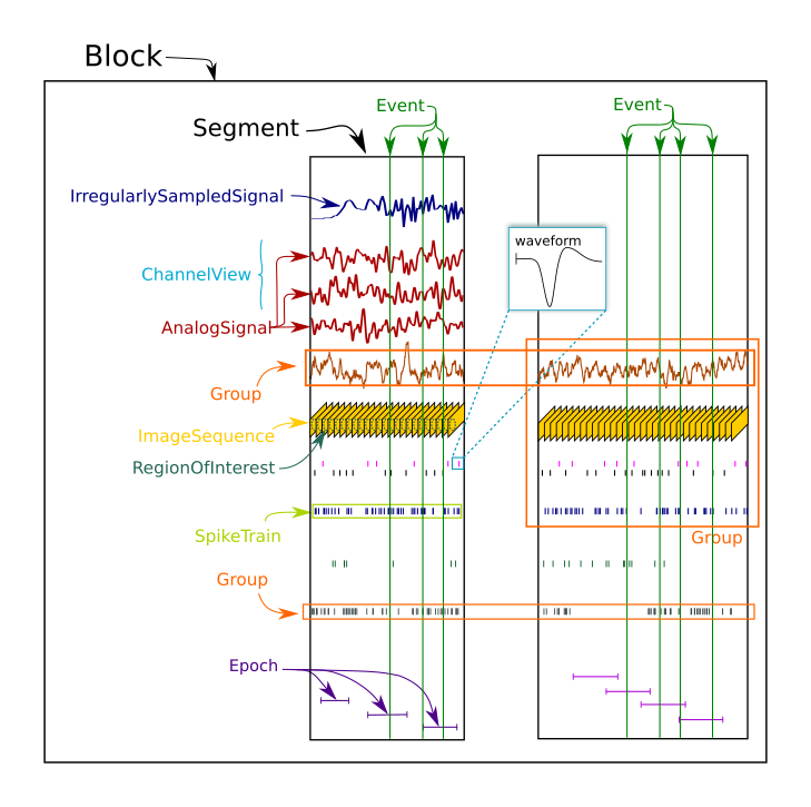
Beyond the core data classes, Neo has various classes for grouping and structuring different data objects.
We have already met two of them, the Block and Segment.
Tree structure#
Block and Segment provide a basic two-level hierarchical structure:
Blocks contain Segments, which contain data objects.
Segments are used to group data that have a common time basis, i.e. that were recorded at the same time.
A Segment can be considered as equivalent to a “trial”, “episode”, “run”, “recording”, etc.,
depending on the experimental context.
Segments have the following attributes, used to access lists of data objects:
analogsignalsepochseventsimagesequencesirregularlysampledsignalsspiketrains
Block is the top-level container gathering all of the data, discrete and continuous, for a given recording session.
It contains Segment and Group (see next section) objects in the attributes segments and groups.
Grouping and linking objects#
Sometimes your data have a structure that goes beyond a simple two-level hierarchy. For example, suppose that you wish to group together signals that were recorded from the same tetrode in multi-tetrode recording setup.
For this, Neo provides a Group class:
In [50]: from neo import Group

In [51]: signal1 = AnalogSignal(np.random.normal(-65.0, 5.0, size=(100, 5)), units=mV, sampling_rate=1 * kHz)

In [52]: signal2 = AnalogSignal(np.random.normal(-65.0, 5.0, size=(1000, 5)), units=nA, sampling_rate=10 * kHz)

In [53]: group = Group(objects=(signal1, signal2))

In [54]: group
Out[54]:
Group with [<AnalogSignal(array([[-60.43622056, -59.80675634, -69.46948022, -65.53666359,
        -60.39588558],
       [-63.1535924 , -67.36457031, -58.54950822, -57.50861782,
        -63.5822156 ],
       [-58.11123152, -62.86463451, -54.92091227, -62.00046628,
        -72.50614004],
       [-61.0528288 , -62.43364966, -64.70212103, -70.3591404 ,
        -62.9466021 ],
       [-57.11836529, -57.06917351, -56.19334658, -58.47575006,
        -68.18614547],
       [-68.47505637, -68.71957508, -74.04820294, -72.75981603,
        -61.4757869 ],
       [-64.45013299, -59.94888427, -62.74054296, -63.98593125,
        -73.42599058],
       [-65.09856253, -64.86569143, -61.50284476, -65.87748779,
        -67.63486107],
       [-61.35352587, -55.18684701, -63.39555601, -67.25107147,
        -68.3935997 ],
       [-73.85896804, -67.04744489, -60.78236   , -61.65190319,
        -68.80664704],
       [-68.48556679, -67.63589956, -67.81178416, -63.46878776,
        -66.55548135],
       [-60.91443834, -60.63074281, -68.50022194, -60.26349079,
        -58.49336377],
       [-62.92597067, -64.23467981, -65.44198016, -60.54702565,
        -70.25076711],
       [-60.16869682, -54.34547162, -64.3213703 , -67.24884929,
        -63.88448983],
       [-57.96804026, -58.44381967, -59.87962649, -71.42071904,
        -56.94371215],
       [-61.13403565, -68.43097426, -57.87107705, -75.68852672,
        -61.31268582],
       [-70.59155002, -67.67266769, -57.0502246 , -60.71302539,
        -61.53523815],
       [-63.32429983, -66.70772263, -56.02106243, -60.92819099,
        -74.55958337],
       [-62.1638982 , -60.02425728, -72.69806199, -69.8571385 ,
        -67.99315092],
       [-65.50066778, -63.09148483, -63.83368633, -68.80252339,
        -68.27454285],
       [-73.49340154, -70.75524263, -62.42062694, -69.65789462,
        -63.84115012],
       [-66.23558055, -60.09924044, -66.91162012, -66.99221665,
        -71.0102535 ],
       [-59.04688742, -62.23016746, -58.31164502, -60.22184577,
        -63.6590791 ],
       [-69.20041884, -54.20263269, -61.27951087, -69.17568707,
        -55.11036603],
       [-64.36405325, -72.22166385, -66.55336018, -61.57292723,
        -67.87652124],
       [-66.05712155, -56.46144061, -62.43975844, -75.08858636,
        -79.33563718],
       [-68.56678551, -58.68519531, -60.45049232, -66.17862148,
        -58.34395661],
       [-63.77611322, -71.36125639, -68.13612845, -61.39074414,
        -62.26959986],
       [-61.75395066, -62.61541832, -65.6007846 , -67.3262752 ,
        -69.94658996],
       [-60.76366576, -64.70740232, -71.8719246 , -58.92536878,
        -63.38495259],
       [-64.99217836, -62.9162623 , -69.2857276 , -69.12811786,
        -65.7726844 ],
       [-69.20099249, -67.44045657, -71.40418161, -53.89567968,
        -70.1117299 ],
       [-66.60052415, -61.09798184, -64.00646407, -67.37793867,
        -57.23448875],
       [-63.65032621, -69.78107934, -63.63159916, -71.47414876,
        -64.43615881],
       [-72.75600228, -72.13562043, -62.48711296, -62.86426955,
        -62.93725858],
       [-58.90219651, -60.14284522, -70.70215353, -60.7567467 ,
        -71.34027031],
       [-65.43001165, -60.09485484, -65.72346458, -62.05875179,
        -57.4811621 ],
       [-70.82774453, -69.76392942, -65.01219287, -64.35365757,
        -64.38859593],
       [-69.67266446, -63.44563651, -69.47318503, -62.94434978,
        -61.09332376],
       [-62.90350382, -65.96044219, -68.56228723, -67.05074974,
        -57.54593786],
       [-66.03435789, -71.69252568, -68.08305805, -74.15842049,
        -59.28451597],
       [-71.57828953, -69.05360985, -67.82654642, -59.94845214,
        -63.78042783],
       [-60.71832847, -69.08600457, -60.26962501, -71.20592852,
        -70.02689296],
       [-63.87122591, -67.30683241, -66.9567411 , -71.87941834,
        -75.42106925],
       [-63.59216845, -68.43421542, -61.70973398, -69.982871  ,
        -63.18092344],
       [-53.18742061, -66.11261604, -64.14656433, -67.6614474 ,
        -75.30318766],
       [-65.68573435, -62.21819633, -70.82035571, -59.20819977,
        -65.67229236],
       [-63.60659201, -64.31072016, -63.61437691, -67.6749363 ,
        -62.32034943],
       [-58.63735749, -65.31877234, -60.53582872, -61.13989636,
        -63.08384986],
       [-71.02068468, -57.23089216, -73.56484076, -68.03703926,
        -57.23437733],
       [-66.55457266, -64.07459168, -66.29818324, -62.6890315 ,
        -78.07655232],
       [-63.44546606, -54.13263537, -65.927585  , -64.08334545,
        -63.25020264],
       [-68.64277486, -62.57622518, -64.6109644 , -62.32247673,
        -72.64293405],
       [-72.90038903, -68.33004742, -58.72824362, -70.51124966,
        -64.6041707 ],
       [-70.52125234, -67.41507564, -63.60339984, -59.10770263,
        -54.7918686 ],
       [-61.67442408, -56.67245323, -69.26725233, -68.6798046 ,
        -76.35933416],
       [-55.30009076, -66.72292813, -59.32208166, -64.76550803,
        -70.82948639],
       [-57.8034028 , -67.26928691, -73.99615575, -56.64737749,
        -60.73068399],
       [-67.89485911, -68.18110261, -61.24427134, -66.61847827,
        -67.90706333],
       [-56.07605374, -62.09195072, -68.79747162, -69.57305183,
        -61.77508323],
       [-55.21016611, -54.41451481, -64.93120076, -67.22564643,
        -61.67210869],
       [-55.34440376, -60.05333382, -70.90744826, -72.63577936,
        -71.94356835],
       [-62.94004888, -62.14024182, -64.89277907, -61.10671075,
        -65.807143  ],
       [-67.69082695, -67.96813296, -70.43314494, -68.5182517 ,
        -77.62551695],
       [-65.50570684, -58.80981626, -66.63566173, -60.55818832,
        -67.24988461],
       [-62.77932165, -65.91659826, -57.84366165, -64.67681504,
        -58.9296617 ],
       [-76.18732573, -65.01579804, -62.18218726, -61.96520023,
        -58.79448153],
       [-61.30803445, -66.31276574, -62.49306328, -61.60006852,
        -69.1961976 ],
       [-58.58027378, -60.56440089, -55.4837794 , -64.42792129,
        -63.2872943 ],
       [-61.73723703, -65.74781442, -68.77384748, -68.23573077,
        -60.47661687],
       [-73.6722787 , -72.18019395, -56.91238021, -59.15177202,
        -66.48064861],
       [-57.79501855, -65.76161034, -65.37084908, -71.61816651,
        -62.977303  ],
       [-73.20005995, -65.04672364, -67.29634749, -70.20032754,
        -74.78466777],
       [-67.37337685, -60.38608848, -58.12184784, -68.49198475,
        -57.02228001],
       [-68.00887787, -51.3670771 , -67.26094556, -63.78154031,
        -64.03371406],
       [-69.49672529, -61.73121122, -74.83552235, -58.52259227,
        -68.11180113],
       [-54.84411962, -62.08846934, -64.47058612, -61.26139436,
        -60.98644615],
       [-70.35684031, -70.58592645, -70.70427358, -55.24418588,
        -64.70652469],
       [-66.52559677, -63.48038036, -55.00183797, -73.49300446,
        -71.52862417],
       [-57.51467396, -67.39283772, -68.29813535, -66.14874577,
        -59.81163289],
       [-65.04093522, -63.62605254, -58.18261656, -60.07037518,
        -63.37356227],
       [-61.1198689 , -66.79423632, -61.48159967, -57.40879978,
        -68.89817062],
       [-73.85162919, -69.31726373, -70.27344881, -70.41260159,
        -68.53099987],
       [-64.15833699, -59.79120457, -66.34294915, -66.85947978,
        -66.53122182],
       [-69.82463694, -61.59221503, -69.01906472, -59.48499746,
        -68.06786259],
       [-68.87475224, -61.12914997, -62.69235188, -67.93371878,
        -63.22395781],
       [-62.81125701, -66.93032998, -67.08274405, -55.28910518,
        -59.55077808],
       [-63.4443415 , -59.93216366, -64.41335579, -68.31391173,
        -69.45919923],
       [-69.07589426, -72.78039099, -53.56545076, -65.88772087,
        -52.64779341],
       [-68.2698611 , -60.76183959, -59.29741165, -67.95083065,
        -72.51665602],
       [-55.89000948, -56.07444896, -63.39163399, -66.18813098,
        -69.93973618],
       [-68.2721513 , -70.75901653, -69.12905928, -58.41446662,
        -57.85937164],
       [-59.44232954, -54.43020506, -68.03827663, -68.71040061,
        -61.39302611],
       [-68.11699512, -57.94927116, -66.17076463, -62.83799795,
        -67.52786839],
       [-58.19206285, -61.96084243, -63.34387504, -70.3665202 ,
        -70.46667273],
       [-64.23113666, -64.74281052, -64.78930237, -64.87238519,
        -63.51661144],
       [-69.26764222, -66.74744275, -60.66629144, -70.07897089,
        -65.57958751],
       [-65.74795366, -63.48176769, -59.60093202, -69.28233152,
        -66.45970571],
       [-64.61891624, -70.11032319, -58.99306251, -66.92736492,
        -59.6564755 ],
       [-64.4399268 , -61.91628304, -66.38417314, -72.07781849,
        -62.98204264]]) * mV, [0.0 s, 0.1 s], sampling rate: 1.0 kHz)>, <AnalogSignal(array([[-60.8962065 , -61.18228932, -63.2737985 , -73.02588965,
        -64.17895659],
       [-68.10183944, -61.62565901, -68.96244523, -63.96604717,
        -63.13536457],
       [-66.31801096, -65.84726248, -62.00072721, -65.24643549,
        -54.52119225],
       ...,
       [-52.41874913, -65.27508057, -54.5733397 , -61.5681143 ,
        -65.83804947],
       [-62.46233662, -69.80067448, -61.70425986, -63.99254951,
        -62.85673774],
       [-73.87031502, -71.24963661, -66.44200687, -72.57036262,
        -73.7111463 ]], shape=(1000, 5)) * nA, [0.0 s, 0.1 s], sampling rate: 10.0 kHz)>] analogsignals
Since AnalogSignals can contain data from multiple channels,
sometimes we wish to include only a subset of channels in a group.
For this, Neo provides the ChannelView class, e.g.:
In [55]: from neo import ChannelView

In [56]: channel_of_interest = ChannelView(obj=signal1, index=[2])

In [57]: signal_with_spikes = Group(objects=(channel_of_interest, spike_train))

In [58]: signal_with_spikes
Out[58]: Group with [<SpikeTrain(array([3., 4., 5.]) * s, [0.0 s, 10.0 s])>] spiketrains, [<neo.core.view.ChannelView object at 0x78725c3d82d0>] channelviews
Performance and memory consumption#
In some cases you may not wish to load everything in memory, because it could be too big, or you know you only need to access a subset of the data in a file.
For this scenario, some IO modules provide an optional argument to their read() methods: lazy=True/False.
With lazy=True all data objects (AnalogSignal/SpikeTrain/Event/Epoch/ImageSequence)
are replaced by proxy objects (AnalogSignalProxy/SpikeTrainProxy/EventProxy/EpochProxy/ImageSequenceProxy).
By default (if not specified), lazy=False, i.e. all data are loaded.
These proxy objects contain metadata (name, sampling_rate, …) so they can be inspected,
but they do not contain any array-like data.
When you want to load the actual data from a proxy object, use the load() method
to return a real data object of the appropriate type.
Furthermore load() has a time_slice argument, which allows you to load only a slice of data from the file.
In this way the consumption of memory can be finely controlled.
Examples#
For more examples of using Neo, see Examples.
Citing Neo#
If you use Neo in your work, please mention the use of Neo in your Methods section,
using our RRID: RRID:SCR_000634.
If you wish to cite Neo in publications, please use:
Garcia S., Guarino D., Jaillet F., Jennings T.R., Pröpper R., Rautenberg P.L., Rodgers C., Sobolev A.,Wachtler T., Yger P. and Davison A.P. (2014) Neo: an object model for handling electrophysiology data in multiple formats. Frontiers in Neuroinformatics 8:10: doi:10.3389/fninf.2014.00010
A BibTeX entry for LaTeX users is:
@article{neo14,
    author = {Garcia S. and Guarino D. and Jaillet F. and Jennings T.R. and Pröpper R. and
              Rautenberg P.L. and Rodgers C. and Sobolev A. and Wachtler T. and Yger P.
              and Davison A.P.},
    doi = {10.3389/fninf.2014.00010},
    full_text = {https://www.frontiersin.org/articles/10.3389/fninf.2014.00010/full},
    journal = {Frontiers in Neuroinformatics},
    month = {February},
    title = {Neo: an object model for handling electrophysiology data in multiple formats},
    volume = {8:10},
    year = {2014}
}