Typical use cases

Recording multiple trials from multiple channels

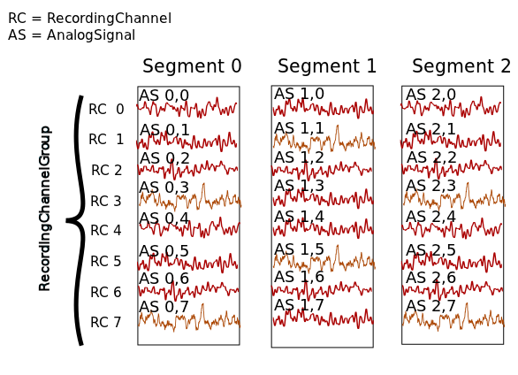
In this example we suppose that we have recorded from an 8-channel probe, and that we have recorded three trials/episodes. We therefore have a total of 8 x 3 = 24 signals, each represented by an AnalogSignal object.

Our entire dataset is contained in a Block, which in turn contains:

• 3 Segment objects, each representing data from a single trial,
• 1 RecordingChannelGroup, composed of 8 RecordingChannel objects.

Segment and RecordingChannel objects provide two different ways to access the data, corresponding respectively, in this scenario, to access by time and by space.

Note

segments do not always represent trials, they can be used for many purposes: segments could represent parallel recordings for different subjects, or different steps in a current clamp protocol.

Temporal (by segment)

In this case you want to go through your data in order, perhaps because you want to correlate the neural response with the stimulus that was delivered in each segment. In this example, we’re averaging over the channels.

import numpy as np
from matplotlib import pyplot as plt

for seg in block.segments:
    print("Analyzing segment %d" % seg.index)

    siglist = seg.analogsignals
    avg = np.mean(siglist, axis=0)

    plt.figure()
    plt.plot(avg)
    plt.title("Peak response in segment %d: %f" % (seg.index, avg.max()))

Spatial (by channel)

In this case you want to go through your data by channel location and average over time. Perhaps you want to see which physical location produces the strongest response, and every stimulus was the same:

# We assume that our block has only 1 RecordingChannelGroup
rcg = block.recordingchannelgroups[0]:
for rc in rcg.recordingchannels:
    print("Analyzing channel %d: %s", (rc.index, rc.name))

    siglist = rc.analogsignals
    avg = np.mean(siglist, axis=0)

    plt.figure()
    plt.plot(avg)
    plt.title("Average response on channel %d: %s' % (rc.index, rc.name)

Note that Block.list_recordingchannels is a property that gives direct access to all RecordingChannels, so the two first lines:

rcg = block.recordingchannelgroups[0]:
for rc in rcg.recordingchannels:

could be written as:

for rc in block.list_recordingchannels:

Mixed example

Combining simultaneously the two approaches of descending the hierarchy temporally and spatially can be tricky. Here’s an example. Let’s say you saw something interesting on channel 5 on even numbered trials during the experiment and you want to follow up. What was the average response?

avg = np.mean([seg.analogsignals[5] for seg in block.segments[::2]], axis=1)
plt.plot(avg)

Here we have assumed that segment are temporally ordered in a block.segments and that signals are ordered by channel number in seg.analogsignals. It would be safer, however, to avoid assumptions by explicitly testing the index attribute of the RecordingChannel and Segment objects. One way to do this is to loop over the recording channels and access the segments through the signals (each AnalogSignal contains a reference to the Segment it is contained in).

siglist = []
rcg = block.recordingchannelgroups[0]:
for rc in rcg.recordingchannels:
    if rc.index == 5:
        for anasig in rc.analogsignals:
            if anasig.segment.index % 2 == 0:
                siglist.append(anasig)
avg = np.mean(siglist)

Recording spikes from multiple tetrodes

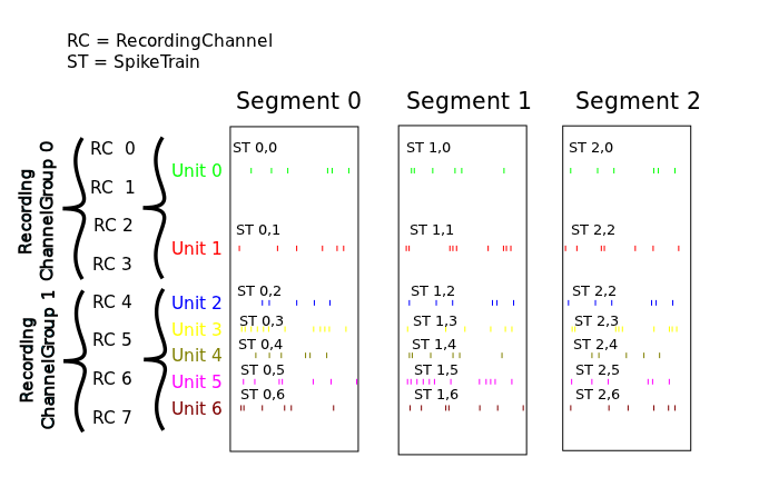
Here is a similar example in which we have recorded with two tetrodes and extracted spikes from the extra-cellular signals. The spike times are contained in SpikeTrain objects.

Again, our data set is contained in a Block, which contains:

• 3 Segments (one per trial).
• 2 RecordingChannelGroups (one per tetrode), which contain:
  • 4 RecordingChannels each
  • 2 Unit objects (= 2 neurons) for the first RecordingChannelGroup
  • 5 Units for the second RecordingChannelGroup.

In total we have 3 x 7 = 21 SpikeTrains in this Block.

There are three ways to access the SpikeTrain data:

• by Segment
• by RecordingChannel
• by Unit

By Segment

In this example, each Segment represents data from one trial, and we want a PSTH for each trial from all units combined:

for seg in block.segments:
    print("Analyzing segment %d" % seg.index)
    stlist = [st - st.t_start for st in seg.spiketrains]
    plt.figure()
    count, bins = np.histogram(stlist)
    plt.bar(bins[:-1], count, width=bins[1] - bins[0])
    plt.title("PSTH in segment %d" % seg.index)

By Unit

Now we can calculate the PSTH averaged over trials for each unit, using the block.list_units property:

for unit in block.list_units:
    stlist = [st - st.t_start for st in unit.spiketrains]
    plt.figure()
    count, bins = np.histogram(stlist)
    plt.bar(bins[:-1], count, width=bins[1] - bins[0])
    plt.title("PSTH of unit %s" % unit.name)

By RecordingChannelGroup

Here we calculate a PSTH averaged over trials by channel location, blending all units:

for rcg in block.recordingchannelgroups:
    stlist = []
    for unit in rcg.units:
        stlist.extend([st - st.t_start for st in unit.spiketrains])
    plt.figure()
    count, bins = np.histogram(stlist)
    plt.bar(bins[:-1], count, width=bins[1] - bins[0])
    plt.title("PSTH blend of tetrode  %s" % rcg.name)

Spike sorting

Spike sorting is the process of detecting and classifying high-frequency deflections (“spikes”) on a group of physically nearby recording channels.

For example, let’s say you have defined a RecordingChannelGroup for a tetrode containing 4 separate channels. Here is an example showing (with fake data) how you could iterate over the contained signals and extract spike times. (Of course in reality you would use a more sophisticated algorithm.)

# generate some fake data
rcg = RecordingChannelGroup()
for n in range(4):
    rcg.recordingchannels.append(neo.RecordingChannel())
    rcg.recordingchannels[n].analogsignals.append(
        AnalogSignal([.1, -2.0, .1, -.1, -.1, -3.0, .1, .1],
            sampling_rate=1000*Hz, units='V'))

# extract spike trains from each channel
st_list = []
for n in range(len(rcg.recordingchannels[0].analogsignals)):
    sigarray = np.array(
        [rcg.recordingchannels[m].analogsignals[n] for m in range(4)])
    # use a simple threshhold detector
    spike_mask = np.where(np.min(sigarray, axis=0) < -1.0 * pq.V)[0]

    # create a spike train
    anasig = rcg.recordingchannels[m].analogsignals[n]
    spike_times = anasig.times[spike_mask]
    st = neo.SpikeTrain(spike_times, t_start=anasig.t_start,
        anasig.t_stop)

    # remember the spike waveforms
    wf_list = []
    for spike_idx in np.nonzero(spike_mask)[0]:
        wf_list.append(sigarray[:, spike_idx-1:spike_idx+2])
    st.waveforms = np.array(wf_list)

    st_list.append(st)

At this point, we have a list of spiketrain objects. We could simply create a single Unit object, assign all spike trains to it, and then assign the Unit to the group on which we detected it.

u = Unit()
u.spiketrains = st_list
rcg.units.append(u)

Now the recording channel group (tetrode) contains a list of analogsignals, and a single Unit object containing all of the detected spiketrains from those signals.

Further processing could assign each of the detected spikes to an independent source, a putative single neuron. (This processing is outside the scope of Neo. There are many open-source toolboxes to do it, for instance our sister project OpenElectrophy.)

In that case we would create a separate Unit for each cluster, assign its spiketrains to it, and then store all the units in the original recording channel group.